What is text mining, and where does it fit?
Text mining, also referred to as text analytics, involves the extraction of insightful information from text, which can help in making well-informed decisions. The method is used in academia (e.g. to analytically understand transcripts that are qualitatively collected), data science (e.g. to produce relevant inputs for predictive modelling), business intelligence (e.g. to improve product, client, marketing, and personnel service). The bottom line is that: text mining is useful where decision is data-driven and text is well-suited as an input.
Why should we care about text mining?
- Social media keeps evolving and affecting an organization’s public efforts.
- An organization’s online content, competitors and external sources, such as blogs, keeps growing.
- Formerly paper records are increasingly digitalized in several legacy industries, such as healthcare.
- Emerging technologies like automatic audio transcription aid in capturing customer touchpoints.
Yet the situation today is that technology companies that are successful pre-dominantly rely on numeric and categorical data in acquiring information, issues of machine learning or in optimizing operations. It does not make sense for an organization to focus only on structured information and, at the same time, invest valuable resources on recording unstructured natural language.
Text largely remains an unused input with competitive advantage. Lastly, there is a shift in companies from an industrial age toward an information age; it is possible to argue that the most successful enterprises are again moving to a customer‐centric age.
Text mining will ease an analyst’s or data scientist’s efforts to comprehend vast
amounts of text. Rather than text mining, it is also possible to simply ignore text sources or merely sample and manually review text.
Case study
Text mining comprises two types: “bag of words” and “syntatic parsing”. Both of them have benefits and weaknesses. I want to demostrate the usefulness of a “bag of words” text mining method.
1. Problem definition and specific goals: Let’s assume we are trying to understand what college students really want from a statistics textbook. We are publishers of such books, and we want to advise authors on what to improve in the next edition of their books. For now, we need to answer the following question: What qualities are listed in the positive and negative comments of the current edition? I will answer this question using Polarity (a simple sentiment scoring).
2. Identify the text that needs to be collected: Andy Field’s textbook, Discovering Statistics Using R, is a popular textbook that covers how to learn statistics using R. Some consumers purchase these books on Amazon and leave comments about the book. These comments are public and inform new buyers’ decision on whether to buy the book or not. Thus, I restricted my data collection to Amazon. After a lot of Googling, I was able to webscrape all reviews on Andy’s book from Amazon webpage using R. But one could expand to other e-commerce companies that sell Andy’s book.
3. Organize the text: I cleaned up the reviews. I organized them to a csv, so we can focus on the specific tasks related to the question.
4. Extract features: Once it is organized, we need to calculate various sentiments and polarity scores.
options(stringsAsFactors = F)
library(tm)
library(qdap)
library(wordcloud)
library(ggplot2)
library(ggthemes)

text.df<-read.csv("Andy_amazon.csv", encoding = 'UTF-8')
text.df$review_text<-iconv(text.df$review_text,"UTF-8" , "UTF-8",
                           "byte")
The next step is to calculate the polarity of each reviewer comment. The scores for each document are within the polarity output, text.df.pol. The element “all” include a scored vector called “polarity”, but it includes more than that information. Both all and polarity should be mentioned to retain only the scores for this particular word cloud. You might want to plot the distribution of the polarity scores , as shown below, before you create a sentiment‐based word cloud.
text.df.pol<-polarity(text.df$review_text)

ggplot(text.df.pol$all, aes(x=polarity,y=..density..)) + theme_gdocs() +geom_histogram(binwidth=.25, fill="darkred",colour="grey60", size=.2) + geom_density(size=.75)
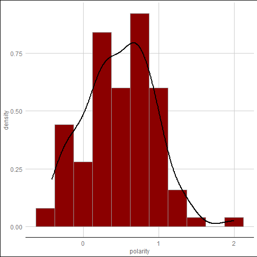
Having calculated the polarity scores, you can now add it to the original data frame. The next code add just the polarity scores from the text.df.pol object to the original text.df data frame. Note that the scale function is applied to the polarity output. You may notice that the polarity scores are not centered at 0 when conducting exploratory data analysis. As shown in the figure above, the mean of the original polarity scores is around 0.48.
summary(text.df.pol$all$polarity)
   Min. 1st Qu.  Median    Mean 3rd Qu.    Max.
-0.4126  0.1677  0.4891  0.4795  0.7917  1.9969
This means that on average each review has at least a single positive word in it. This occurs alot in reviews and market research. Despite anonymity, people normally tend to be nice or say something postive. That is, there is a tendency that they mix positive words with negative ones. By scaling the polarity score vector, one can move the mean to zero. One should use the scale function and try to do the analysis again without it to get a sense of how the scaling affect outcomes.
text.df$polarity<-scale(text.df.pol$all$polarity)
ggplot(text.df, aes(x=polarity,y=..density..)) + theme_gdocs() +geom_histogram(binwidth=.25, fill="darkred",colour="grey60", size=.2) + geom_density(size=.75)

5. Analyze: The sentiment and polarity scores are used to subset the reviews foe the analysis of the terms used distinctly in positive or negative comments. For the creation of the sentiment‐based word cloud, a subset of the original data needs to be created. This will ensure that one has only the positive or negative documents. To get this, one can apply the subset function as described in the code.
pos.comments<-subset(text.df$review_text,
                     text.df$polarity>0)

neg.comments<-subset(text.df$review_text,
                     text.df$polarity<0)

pos.terms<-paste(pos.comments,collapse = " ")
neg.terms<-paste(neg.comments,collapse = " ")
all.terms<-c(pos.terms,neg.terms)
all.corpus<-VCorpus(VectorSource(all.terms))

all.tdm<-TermDocumentMatrix(all.corpus,
                            control=list(weighting=weightTfIdf, removePunctuation =
                                           TRUE,stopwords=stopwords(kind='en')))

all.tdm.m<-as.matrix(all.tdm)
colnames(all.tdm.m)<-c('positive','negative')

comparison.cloud(all.tdm.m, max.words=100,title.size=2,
                 colors=c('darkgreen','darkred'))

comparison.cloud(all.tdm.m, max.words=100,title.size=2,
                 random=FALSE, scale=c(2,0.5),
                 colors=c('darkgreen','darkred'))
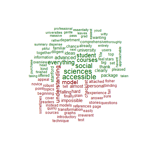
6. Reach an insight or recommendation: By the end of the case study, you hope that you are able to answer the question from step 1: What qualities are listed in the positive and negative comments of the current edition?
In the positive portion (colored green) of Andy’s book review, words such as advanced, easiest, accessible, approachable, social sciences, were used. One could conclude that to have a positive review especially among social science students, advanced statistics textbook need to be accessible and easy to understand. In contrast, it seems that Andy’s textbook is not designed for advanced user of statistics, as the negative portion (colored red) is characerized by words such as novice, introductory, personal, stories. In his book, Andy tends to tell stories while explaining statistical concepts. This is frawned upon by some users. Taken collectively, Andy’s book is much more useful to not-advanced users of statistics, as it makes statistics accessible. But in the next edition, he should probably reduce the amount of (personal) stories he tells. Such stories perhaps do get in the way of understanding the material.
Source
I learnt the basics of text mining from the book of Ted Kwartler.