Regression discontinuity design (RDD) is a quasi-experimental method for causal inference. RDD has become a prominent method for causal inference since the 2000s. One can account for both observed and unobserved heterogeneity. We can leverage our knowledge of treatment assignment to estimate the effect of a treatment, such as policy, an intervention, on an outcome. Like matching, the aim is to identify the effect of a (binary) treatment on the outcome.
But it varies from the other methods in that we take a (running) variable V, in which at some point, there is a qualitative difference between observations with higher and lower values. The running variable is also known as the forcing variable, at which there is a cut off score. A person who lies below this cut-off point doesn’t receive the treatment and a person who lies above the cut-off point recieve the treatment – or vice-versa.
For example, suppose we are interested in the effect of scholarship on students’ grade performance. How can we decide those who get the treatment (here: scholarship) and those who do not get it? We could use a test/exam. The test has a minimum score of 0 and a maximum score of 1000. Those who get at least a 600 get the scholarship and those who get below 600 don’t get it. Here, the running variable is the test score achieved by the students. The cut-off point is 600.
But it is important to note that for people that have very similar scores on any of the specified covariates, the difference between them is random (the error component). In other words, there is no systematic difference between the person who got 590 or a person who got 600 on any of the specified covariates. It is probably just by chance that one knew a question slightly better than the other. In general, there might be some systematic differences between people at the lower and the upper end of the scale. For example, there is a difference in skill between people who had a 200 and those who had a 900. But the difference between people who had 599 or 600 is purely due to chance. But because you need a 600 to get the scholarship, only one of these two persons, who are otherwise more or less the same, gets the scholarship.
To summarize briefly, those individuals that are at the threshold or arbitrarily close to the threshold could have gone either way (there are no systematic difference between the groups except that by chance one got the treatment and the other one didn’t). Therefore, at the cut-off point, we have a scenario that mimics a random allocation into treatment and control group. The implication of this assumption is that we can look at the difference between the two groups on the dependent variable (outcome) and say that the difference between them is due to the treatment. This is Local Average Treatment Effect (LATE). It is local because we are talking about the average treatment effect for those individuals that are close to the threshold.
Case study
Problem definition and specific goals
Let’s do a (simple) reproduction of David Szakonyi (APSR, 2017) that used regression discontinuity to estimate the effect of political connections on firm performance. The study examined whether businesspeople who become legislators are able to secure benefits for their firms while serving in elected office. The RQ is: Do businesspeople who win elected office use their positions to help their firms?
Note: The R codes I used are different from the one used in the original study. These R codes, adapted from the code of Bauer and Cohen’s online chapter on RDD, make me focus on the general idea and aim of RDD, as I learnt it.
Data collection
Szakonyi included in the sample all companies with a director, deputy director, board chair, or board member campaigning to be elected to office in a single-member district (SMD). The treatment is electoral victory, which is assigned a value of 1 if a firm is associated with a winning candidate and 0 otherwise. The running/forcing variable used is vote margin, which takes values from -1 to 1 and the cutoff point is set at zero. More specifically, firms that are connected to winning candidates (the treatment group) have positive signs. But, firms connected to losing candidates (the control group) have negative signs.
The outcome is logged total revenue measured in millions of rubles, and profit margin. The study examines elections to 114 regional parliamentary convocations in 78 sub-national units of Russia from the 1st of January 2004 to the 3rd of March 2011.
Organize data and extract features
library(ggplot2)
load(file="Candidates.Rdata")
load(file="ConnectedFirms.Rdata")
Before carrying out any statistical analysis, I will check if there is any sign of manipulation of the running variable. For the validity of RDD estimation (i.e. produce LATE estimate that is unbiased at the cutoff ), it is vital that the eligibility index has not been manipulated close to the cutoff. This manipulation can occur in variety of ways. In my introductory example, the students who take the tests for scholarships may purposefully cheat if they think that doing so would make them pass the aptitude test for the scholarship.
We can check the density of the running variable as a kind of falsification test. If the density (the number of observations) below cutoff significantly varies from the one above, it might be the case that individuals/politicians/parties in districts can manipulate their scores. The easiest thing to do is to show a histogram of the running variable using a large number of bins. Check the distribution of the margin of victory and play around with the binwidth. While it is advisable to make the binwidth very small, it should still be possible to visualize the overall pattern of the distribution. The idea here is to see if you can identify irregularity right at the zero margin. Depending on the binwidth you use, you might observe strange things happening, e.g. a sudden drop after zero, which means we might have self-selection. But if there is considerable variation everywhere, it’s probably not an issue.
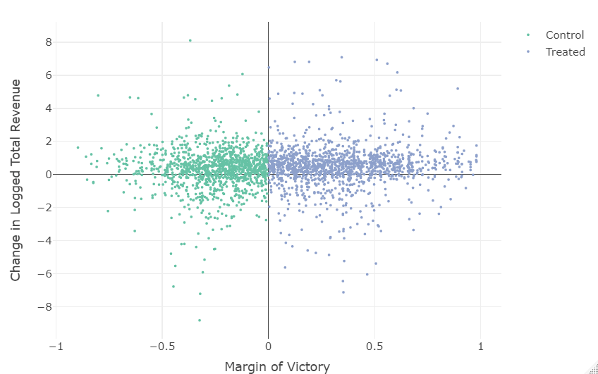
# Plot outcome variable vs. running variable
library(plotly)
cons$colour[cons$margin<=0] <- "Control"
cons$colour[cons$margin>0] <- "Treated"

plot_ly(data = cons,
        type = "scatter",
        mode = "markers",
        x = cons$margin,
        y = cons$fullturnover.e.l.d,
        color = cons$colour,
        marker = list(size=3)) %>%
  layout(xaxis = list(title = "Margin of Victory", dtick = 0.5),
         yaxis = list(title = "Change in Logged Total Revenue"))
# histogram of density test
p = ggplot(cons,aes(x=margin, fill = factor(cons$margin>0)))+
  geom_histogram(binwidth=0.02)+xlim(-1,1)+geom_vline(xintercept = 0)+
  xlab("Change in Logged Total Revenue")+scale_colour_manual(values = c("red","blue"))+
  theme_bw()+theme(legend.position='none')
p

Formally, we can use certain procedures, such as RDD density, to test the existence of manipulation of the running variable at the cut-off. More specifically, it is a test of the null hypothesis that there is no discontinuity. If there is no manipulation, then the density of the running variable ought to be continuous close to the cut-off.
The output suggests that at the cut-off 0, there is no sign of manipulation because the null hypothesis is not rejected (the p-value is 0.07). So, there is no self-selection or sorting of units into the treatment around the cut-off.
library(rddensity)
summary(rddensity(X = cons$margin, vce="jackknife"))
Manipulation testing using local polynomial density estimation.

Number of obs =       2806
Model =               unrestricted
Kernel =              triangular
BW method =           estimated
VCE method =          jackknife

c = 0                 Left of c           Right of c
Number of obs         1332                1474
Eff. Number of obs    448                 409
Order est. (p)        2                   2
Order bias (q)        3                   3
BW est. (h)           0.157               0.172

Method                T                   P > |T|
Robust                -1.7975             0.0723
Ideally, you should also verify whether you have a sharp or fuzzy discontinuity. If units fully comply with their treatment assignment, you have a case of sharp discontinuity and a fuzzy discontinuity otherwise. In this case study, I should have tested whether the elected offices were indeed associated with the winning businesspeople.
Analysis
Now let’s estimate the result. We can use the rdrobust function to get the RDD estimate. Simply run the outcome variable on the running variable, which runs from -1 to 1, where cut off is at 0. Thus, it will estimate at zero. The cut off is, by default, zero if not set.
The result below shows information about the numbers of observation on each side of the cut-off and the order of the fitted polynomials.
library(rdrobust)
set.seed(48104)
fit <- rdrobust(cons$fullturnover.e.l.d, cons$margin, c = 0, all=TRUE)
summary(fit)
Call: rdrobust

Number of Obs.                 2568
BW type                       mserd
Kernel                   Triangular
VCE method                       NN

Number of Obs.                1185        1383
Eff. Number of Obs.            343         314
Order est. (p)                   1           1
Order bias  (q)                  2           2
BW est. (h)                  0.138       0.138
BW bias (b)                  0.260       0.260
rho (h/b)                    0.530       0.530
Unique Obs.                    892         855

=============================================================================
        Method     Coef. Std. Err.         z     P>|z|      [ 95% C.I. ]
=============================================================================
  Conventional     0.548     0.197     2.777     0.005     [0.161 , 0.934]
Bias-Corrected     0.619     0.197     3.136     0.002     [0.232 , 1.005]
        Robust     0.619     0.225     2.746     0.006     [0.177 , 1.060]
=============================================================================
You usually also plot the data. Below is a RDD plot using the whole data range. A comparison of the mean outcomes to the left and right of the cut-off point shows the degree of the treatment effect. We see evidence of a discontiniuty at the cut-off point in the graph.
rdplot(cons$fullturnover.e.l.d,cons$margin,
       x.lab="Margin of Victory",
       y.lab="Change in Logged Total Revenue",
       title = "RDD Estimate")

An increase in the lengths of the bin might induce bias to the estimates because they are just averages and do not take into account the slope in the mean outcome functions. Also, wide bins undermines the credibility of the comparison of both sides of the cut-off because the comparison is no longer restricted to electoral victory just around the cut-off.
How do we make the right selection of bandwidth around the cut-off? The bandwidth should be sufficiently broad to include an adequate number of observations and get precise estimates. It should also be sufficiently narrow to compare similar units and minimize selection bias. There are variety of ways to choose the bandwidth. We can use the command fit$bws to choose the optimal bandwidth. The result suggests that the optimal bandwidth is approximately 0.138.
fit$bws
      left     right
h 0.1378813 0.1378813
b 0.2600304 0.2600304
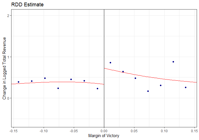
The RDD treatment estimate will be computed and plotted using this bandwidth, where x axis is restricted to (-0.14, 0.14).
Below, the RDD treatment effect/point estimate is 0.547 and p< 0.05. Thus, there is enough evidence at the 0.05 level of significance to support the claim that when a businessperson from a company barely wins an election to a state legislature, the revenue of the company in the next year will be 0.547 larger than if they didn’t.
The output also includes confidence intervals. The third one is called the robust confidence interval. This takes into consideration that RDD uses polynomials to estimate the underlying mean outcome functions. The variance is corrected for the misspecification error or smoothing bias. When samples are particularly small, it should be used for testing the statistical significance of a treatment effect.
summary(rdrobust(cons$fullturnover.e.l.d, cons$margin, h=0.138,all=TRUE))
Call: rdrobust

Number of Obs.                 2568
BW type                      Manual
Kernel                   Triangular
VCE method                       NN

Number of Obs.                1185        1383
Eff. Number of Obs.            343         314
Order est. (p)                   1           1
Order bias  (q)                  2           2
BW est. (h)                  0.138       0.138
BW bias (b)                  0.138       0.138
rho (h/b)                    1.000       1.000
Unique Obs.                    892         855

=============================================================================
        Method     Coef. Std. Err.         z     P>|z|      [ 95% C.I. ]
=============================================================================
  Conventional     0.547     0.197     2.776     0.006     [0.161 , 0.934]
Bias-Corrected     0.855     0.197     4.339     0.000     [0.469 , 1.242]
        Robust     0.855     0.317     2.697     0.007     [0.234 , 1.477]
=============================================================================
rdplot(cons$fullturnover.e.l.d,cons$margin,x.lim=c(-0.14,0.14),
       x.lab="Margin of Victory",
       y.lab="Change in Logged Total Revenue", title = "RDD Estimate")
Finally, when implemenenting RDD, you should carry out sensitivity test so you know if your result are significantly sensitive to different specifications. Examine if the RDD estimates are robust to variety of bandwidths as well as the use of higher-order polynomial terms. If your treatment effect goes away (i.e., becomes insignificant and/or looks too different) with the use of a higher-order polynomial, this means your result is too sensitive and not credible.
Another type of senesitivity test is robustness check. This involves testing whether there are jumps in the dependent variable at other placebo cut-offs. There should be treatment effect at the treatment assignment cut-off. But we shouldn’t see similar jumps at other levels of the running variable without a logical explanation behind it.
Let’s test the treatment effect at the placebo thresholds/cutoffs. In both placebo cut-off points below, the treatment effect is not significant at the 0.05 level of signifcance.
First placebo cut-off:
# cutoff c = 0.25
placebo <- rdrobust(cons$fullturnover.e.l.d, cons$margin, c = 0.25, all=TRUE)
summary(placebo)
Call: rdrobust

Number of Obs.                 2568
BW type                       mserd
Kernel                   Triangular
VCE method                       NN

Number of Obs.                1742         826
Eff. Number of Obs.            450         411
Order est. (p)                   1           1
Order bias  (q)                  2           2
BW est. (h)                  0.196       0.196
BW bias (b)                  0.291       0.291
rho (h/b)                    0.674       0.674
Unique Obs.                   1251         496

=============================================================================
        Method     Coef. Std. Err.         z     P>|z|      [ 95% C.I. ]
=============================================================================
  Conventional     0.022     0.200     0.112     0.911    [-0.370 , 0.414]
Bias-Corrected     0.034     0.200     0.168     0.867    [-0.358 , 0.425]
        Robust     0.034     0.238     0.141     0.888    [-0.434 , 0.501]
=============================================================================
Second placebo cut-off:
# cutoff c = -0.30
placebo1 <- rdrobust(cons$fullturnover.e.l.d, cons$margin, c = -0.30, all=TRUE)
summary(placebo1)
Call: rdrobust

Number of Obs.                 2568
BW type                       mserd
Kernel                   Triangular
VCE method                       NN

Number of Obs.                 405        2163
Eff. Number of Obs.            234         339
Order est. (p)                   1           1
Order bias  (q)                  2           2
BW est. (h)                  0.130       0.130
BW bias (b)                  0.207       0.207
rho (h/b)                    0.625       0.625
Unique Obs.                    323        1424

=============================================================================
        Method     Coef. Std. Err.         z     P>|z|      [ 95% C.I. ]
=============================================================================
  Conventional     0.309     0.303     1.020     0.308    [-0.285 , 0.904]
Bias-Corrected     0.435     0.303     1.434     0.152    [-0.160 , 1.030]
        Robust     0.435     0.359     1.211     0.226    [-0.269 , 1.139]
=============================================================================
Conclusion
From this case study, we can conclude that businesspeople who become legislators are able to secure benefits for their firms while serving in elected office.
Even though researchers are not in control of treatment assignment in RDD, as they are in randomized controlled trial (RCT), treatment assignment depends on observable characteristics of the world that are verifiable. In contrast to other quasi-experimental methods, we can objectively evaluate the assumptions needed to use this method.
Finally, although RDD produces an unbiased estimate of the treatment effect at the discontinuity, it yields Local Average Treatment Effect (LATE), which might sometimes not be generalizable or interesting.
References
Gertler, P. J., Martinez, S., Premand, P., Rawlings, L. B., & Vermeersch, C. M. (2016). Impact evaluation in practice. The World Bank.
Paul C. Bauer and Denis Cohen. Chapter 13 RDD: Regression Discontinuity Design
PEP online course: Evaluation of Public Policies: Class 10: Regression Discontinuity
Szakonyi, D. (2018). Businesspeople in elected office: Identifying private benefits from firm-level returns. American Political Science Review, 112(2), 322-338.
