Natural Experiment
Before discussing natural experiment, it makes sense to explain randomized assignment. By this, I mean that we randomly assign eligible units (or observations) to either a treatment or a control group. Due to the random assignment, there is a 50-50 chance for each eligible observation to be selected, which leads to an internally valid causal estimates. Randomization can also result in the achievement of statistical independence, which minimizes the risk of omitted variable bias or endogenity. Statistical independence implies that there is no correlation between the treatment variable and the other variables. In sum, the key assumption is that randomization effectively generates two groups that are statistically similar as to the observed and unobserved characteristics.
However, randomization are sometimes infeasible because the subject we study are not amenable to an experiment. Also, experimental designs could sometimes be unethical, or too costly.
So, the intuition behind Natural Experiments and Instrumental Variable (IV) is to mimic randomization by taking advantage of some external source of variation to determine treatment status. To identify the effect of a treatment on an outcome, we search for events that are (close to) random (i.e., bring about random variation in the independent variable). We use this random phenomena as a source of randomization. To summarize briefly: Rather than actually conducting an experiment, we use events or policies that randomly take place as a source of exogenous variation in our variable of interest.
Example from Social Science
In their 2008 article published in The Scandinavian Journal of Economics, Monstad, Propper and Salvanes (called MPS from now on) were interested in the impact of education on fertility. Looking back to my introduction to statistics class, one naive way I would have used in carrying out the analysis is to simply regress FERTILITY on EDUCATION and other variables:
FERTILITY= Β0 + Β1EDUCATION + Β2 X2 +Β3 X3 + Βn Xn + error
where fertility is the outcome (the timing and number of children as well as childlessness, wherein the first and third variables are binary). EDUCATION refers to the obtained number of years of education.
If we found a negative slope, this might seem to support the hypothesis that there is a causal link between fertility and education. But EDUCATION is not randomly assigned. So, it would be endogenous. Therefore, there would be omitted variable bias in Beta1 hat. So, we can’t simply run the regression because this will result in a biased estimate of Beta1 hat, which does not represent the true impact of EDUCATION on FERTILITY.
So, I guess that’s why MPS didn’t execute such a naive analysis. But how can we resolve this issue? Let’s discuss two solutions:
Solution 1: Randomized Selection
Randomized experiment: In theory, we can randomly assign education level to the subjects (here: women). That is, we would find women with low level of education, then randomly assign half to receive higher level of education and the other half to not. Then, at some point, we could measure the impact of having an additional level of education on FERTILITY. If persons with a randomly assigned higher level of education have declining fertility, this would demonstrate evidence that education level has a negative impact on fertility. But it’s unethical to do this!
Solution 2: Natural Experiment
We find some source of natural random variation in educational level (mimic randomization) and use that instead of an actual experiment. Such variation or exogeneity can come from the time a particular government policy came into effect.
In their article, MPS used a policy change in Norway as a natural experiment to study the impact of education on fertility. During the 1960s in Norway, there was a far-reaching change in the compulsory schooling legislation which affected primary and middle schools. Before the reform, children had to go to school until the seventh grade according to the Norwegian education system. After the reform, however, the length of school attendance was extended to the ninth grade, which meant two additional years of compulsory schooling. These reforms had a profound impact on educational attainment.
The implementation of the reform occurred not only in different municipalities but also at different times. It started in 1960 and continued through 1972. Consequently, this led to variation in the minimum years of schooling at the municipal level and across time. Thus, one can leverage the introduction of this new policy to carry out a natural experiment. In short, the source of exogenous variation in mothers’ education is the education reform in Norway that resulted in an increase in the number of years of compulsory schooling from seven to nine years. It was implemented over a period of 12 years from 1960 to 1972 across different municipalities and over different times.
MPS had a sample of all women given birth to between 1947 and 1958. They determined whether women were influenced by the changed schooling law by linking each woman to the municipality she grew up in. Such connection was possible due to the matching of the administrative data to the 1960 census. This census provided them with the information of the municipality where the woman’s mum lived in I960. The women in their analysis are, in 1960, within the age of two and 13 years. The indicator is coded one for a woman if by the age of 13 (the seventh year of schooling), the new system had come into effect in her municipality of residence, conceived as the place her mother resided in 1960.
In my view, it is safe to assume that women in either side of the municipalities are on average identical. However, women in certain municipalities have access to higher education. MPS were able to exploit that difference as a source of exogenous variation in years of schooling.
MPS then examined fertility of this generation through 2002. That is, in 2002 they observed the children in their sample. By that date, the women that were the youngest in the sample were already aged 44 (By this, I refer to those born in 1958). Therefore, they could observe the complete fertility history for most in the sample. Using the year and month of birth of the children and mother, MPS could deduce the age of the mother (at the time of giving birth) to the nearest month.
The dataset used by MPS is not publicly available. But regarding estimation, econometric analysis using a natural experiment could easily be conducted through the natural random “treatment” variable (REFORM) instead of the independent variable of interest (EDUCATION).
FERTILITY = Β0+ Β1REFORM +Β2 X2 +Βn Xn + error
In this situation, we replaced the endogenous variable of interest (EDUCATION) with a variable that is, as close as possible, randomly assigned by a policy intervention. In other words, we leveraged this policy change to mimick randomization. Instead of using EDUCATION, we use REFORM as our natural treatment variable. REFORM is coded 1 if the individual was affected by the education reform and 0 otherwise. This model is likely to provide us with an unbiased estimate of the impact of education of women on fertility outcome.
This approach can be compared to the estimation of the Intention-to-Treat (ITT) from a randomized experiment under imperfect compliance. ITT is the difference in outcomes between the subjects that receive the treatment condition and the subjects that get the control condition, regardless of whether the subjects given the treatment status actually receives the treatment. Take the reform in Norway for example: it is imaginable that there may have been selective migration into or out of municipalities that implemented the reform early. This is comparable to imperfect compliance (discussed later). Using the natural experiment approach without considering this may cause one to underestimate the true effect, just as with the ITT. However, MPS argued, probably because of this concern, that because the reform implementation did not take place prior to 1960, reform-induced mobility should not be problematic.
Instrumental Variable
These natural treatment variables are commonly employed as instrumental variables. How the instrumental variable approach functions is similar to how the natural experiments work because, for estimation of effect, the IV method depends on an external source of variation that affect treatment condition. IV helps us assess causal effects in cases of imperfect compliance, voluntary enrollment, or universal coverage. The task with the instrumental variable approach is to find an exogenous variable that is highly correlated with the endogenous treatment variable. We then use the exogeneous status of this other variable to identify the treatment effect.
Intuitively, an IV is something beyond the control of the individual that affects their likelihood of getting the treatment, but is not related to their other characteristics. Remember the intuition: if the treatment variable is not randomly assigned it is likely to be “endogenous.” (Endogenous = correlated with the error term). Therefore, the risk of having omitted variable bias is higher. What if there is a possibility to find a variable that is correlated with the treatment but is not associated with the error term? This could be used as a way to assess the causal estimate of the treatment. Such a variable is called an “instrument” or “instrumental variable” or “IV.”
Going back to the article of MPS:
FERTILITY= Β0 + Β1EDUCATION + Β2 X2 +Β3 X3 + Βn Xn + error
EDUCATION will be endogenous in the above-equation. Therefore, there will be omitted variable bias in this regression. We can try to solve this by looking for a variable, say Z, that is highly associated with EDUCATION but is exogenous. Here, Z would be the instrumental variable (IV). In MPS article, whether a woman was affected by the education REFORM or not could be used as an instrumental variable because it is correlated with women years of schooling, but it is, itself, exogenous in that whether a woman is affected by the reform or not is kind of random.
Compliance
Compliance refers to how units respond to the treatment condition. Full compliance with treatment means that all units to whom the treatment has been assigned actually receive the treatment, and those in the comparison units do not receive it. In this scenario, it is safe to say that we are estimating the average treatment effect (ATE) for the population. In reality, on the issue of treatment assignment, potential participants can decide whether to get the treatment or not. The bottomline is that full compliance with treatment and control conditions selection criteria, although desired, is not that common in relation to other experimental settings such as laboratory experiments. So, no matter how much policy makers and evaluation teams try, full compliance to treatment and control status is sometimes not feasible.
Now, we will go through variety of cases that can take place and discuss implications for the use of evaluation methods. But note that the optimal solution to imperfect compliance is simply to avoid it when possible. In this sense, one should strive to keep compliance as high as one can in the treatment group and as low as possible in the comparison group.
Concerning the effect of the instrument in the treatment variable, we have 4 kinds of people:
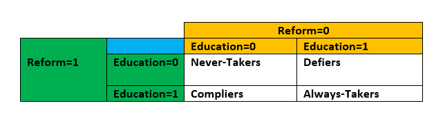
- Always-Takers: This person receives the treatment irrespective of the instrument. In MPS article, this would be women who received additional years of schooling regardless of whether the reform had been implemented in their municipality or not (EDUCATION=1, regardless of REFORM).
- Never-Takers: This individual never gets the treatment regardless of the instrument. In MPS article, this would be women who did not receive additional years of schooling irrespective of whether the reform had been implemented in their municipality or not (EDUCATION=0, regardless of REFORM).
- Compliers: This person receives the treatment only when the instrument induces them to. In MPS article, this would be women who receive additional years of schooling if the reform had been implemented in their municipality (EDUCATION=1, REFORM=1; EDUCATION=0, REFORM=0)
- Defiers: This individual receives the treatment only in cases where the instrument does not require them to. In MPS article, this would be women who did not receive additional years of schooling if the reform had been implemented in their municipality (EDUCATION=0, REFORM=1) but receive additional years of schooling if the reform had not been implemented in their municipality (EDUCATION=1, REFORM=0)
One should consider carefully what type of treatment effect one estimates and their respective interpretation in cases of noncompliance. A first option is to estimate a direct comparison of the group that are initially assigned to treatment with the group initially assigned to the control; this will give us the ITT estimate. The ITT is a comparison of those whom we intended to treat (those assigned to the treatment group) with those whom we intended not to treat (those assigned to the control group). The ITT is a weighted mean of the outcomes of participating subjects and non-participating subjects in the treatment group compared with the mean outcome of the control group. If the noncompliance occurs only on the side of the treatment, the result can still be an appropriate measure of impact because those assigning subjects into treatment conditions cannot force the treatment on their target population.
A second option is to estimate the local average treatment effect (LATE). The remaining part of this post is about how to estimate LATE. The LATE estimation principles is applicable in cases of noncompliance in the treatment group, control group, or both at the same time. In other words, compliance is what comes to mind when assessing the causal effect. The Treatment-on-the-treated (TOT) is a LATE when we specifically have noncompliance only in the treatment group. LATE computes the difference in outcomes between those that actually receive the treatment and the control group. In case of noncompliance in both the treatment and control group, the validity of the LATE estimate is confined to those in the treatment group who received the treatment condition and who would have not received it had they been assigned to the control group.
In sum, the use of an instrumental variable paves the way for identifying the impact of the treatment on compliers. This is known as the local average treatment effect or LATE. The LATE is the effect the treatment has on those who comply with the instrument. In the MPS article, it would be the effect of additional years of schooling on fertility on women affected by the reform only because they reside in municipalities that had implemented it.
We need to make three main assumptions for IV to hold:
- Relevance: The IV is not only correlated with the treatment variable, but also the IV has a causal effect on the treatment variable.
- Independence: The IV is not correlated with the error term i.e. it is not vulnerable to omitted variable bias.
- Exclusion Restriction: The IV has no direct effect on the outcome variable. Its effect on the dependent variable happens through the treatment variable.
But we also need an additional assumption for the LATE to hold:
4. Monotonocity (no deniers): Everyone in the sample received the treatment because they received the instrument. Although this is a logical assumption to make, it relies on intuition.
Case Study: Does Education affect Wages?
Problem Definition and Specific Goal
Using the example (and explanations) from Hill et al. (2018) and R codes from Colonescu (2016), we want to examine if a person’s wage is partly shaped by his or her level of education. Below, you find a log-linear regression model that explains observed hourly wage as:
ln(WAGE) = Β0+ Β1EDUCATION +Β2 EXPER +Β3 EXPER2 + e
with EDUC = years of education and EXPER= years of experience. What else, besides what has been included in the equation, could affect wages? There are numerous factors that we can come up with. According to Hill et al. (2018), such factors include labor market conditions, region of the country, and union membership. However, Hill and colleagues posit that labor economists are mainly worried about the omission of a variable that measures ability. A person’s ability (and industriousness), they argue, may affect their work quality and wage. These variables are part of the error term e. It is, after all, difficult to measure them.
Another challenge is that not only might ABILITY influence WAGES, but also abled individuals may devote additional years to studying in school, which can cause a positive association between the error term e and the education variable EDUC. In that case, the least squares estimator of the divdends to an additional year of education will be biased positively and inconsistent. The bias will remain even in very large samples.
For this reason, we use IV estimation method:
Data Collection
I will use Thomas Mroz’s data on married women in the file mroz.dat made available by Constantin Colonescu (2016).
Extract Features
As Hill et al. (2018) explain, some individuals in the sample do not belong to the labor force and, for this reason, have zero wages. The implication is that one cannot calculate their log. Therefore, it is logical that they exclude such observations and take those for which lpf is 1. Like Hill et al. (2018) and the R codes of Colonescu (2016), we use the N= 428 women in the sample who are part of the labor force.
library(PoEdata)
library(AER) # for "ivreg()"
library(lmtest) # for coeftest()
library(broom)
library(knitr)
library(stargazer)

data("mroz", package="PoEdata")
mroz1 <- mroz[mroz$lfp==1, ] # restricts sample to lfp=1
Analysis
To conduct an instrumental variable estimation, we need a variable that is not part of the wage equation itself but has a correlation with EDUC. However, the variable should not be correlated with the omitted variables that constitute the error term – here, a person’s ability, or intelligence. It is not easy to obtain such variables, but in Thomas Mroz’s data, there is information on the number of schooling years for the woman’s mother. A mother’s education (MOTHEREDUC) is, itself, not part of the daughter’s wage equation. It also makes sense that mothers that are more educated are more likely to have daughters that are more educated. It remains to be seen whether the ability and intelligence of a woman are associated with her mum’s education. For us to have valid instruments, it is necessary that these variables are uncorrelated. This is the assumption that Hill et al. (2018) made.
Hill et al. (2018) used a regression model called Two Stage Least Squares (2SLS) for the IV analysis. It is called 2SLS because it is based on a 2-stage approach. This provides us with an estimate of the treatment on the outcome that is unbiased.
The first stage targets the first causal chain. Here: MOTHEREDUC –> EDUC. The explanatory variables in the first stage equation has all the exogenous variables (controls) of the original equation as well as external instrumental variables.
educ.ols <- lm(educ~exper+I(exper^2)+mothereduc, data=mroz1)
This will give us (least squares) estimates. The fact that MOTHEREDUC is exogenous should provide us with an unbiased estimate of the effect of MOTHEREDUC on EDUC.
educ.ols
Call:
lm(formula = educ ~ exper + I(exper^2) + mothereduc, data = mroz1)

Coefficients:
(Intercept)        exper   I(exper^2)   mothereduc
   9.775103     0.048862    -0.001281     0.267691
kable(tidy(educ.ols), digits=4, align='c', caption=
        "First stage in the 2SLS model for the 'wage' equation")
Table: First stage in the 2SLS model for the 'wage' equation

|    term     | estimate | std.error | statistic | p.value |
|:-----------:|:--------:|:---------:|:---------:|:-------:|
| (Intercept) |  9.7751  |  0.4239   |  23.0605  | 0.0000  |
|    exper    |  0.0489  |  0.0417   |  1.1726   | 0.2416  |
| I(exper^2)  | -0.0013  |  0.0012   |  -1.0290  | 0.3040  |
| mothereduc  |  0.2677  |  0.0311   |  8.5992   | 0.0000  |
As you can see, the coefficient of MOTHEREDUC is highly significant with a t-value of 8.6. This corresponds to an F-test value of 73.95. This result indicates that our
instrument is correlated with the variable we conceived as “suffering” from endogeneity, despite controlling for the remaining exogenous variables in the model.
In Stage 2, which is known as the “Reduced Form”, we use the predicted treatment variable that has now been generated. More specifically, we get the predicted values of education from the first stage equation, EDUC hat, and put it into the log-linear wage equation as a substitute for EDUC. After this, we estimate the equation using least squares:
educHat <- fitted(educ.ols)
wage.2sls <- lm(log(wage)~ educHat+ exper + I(exper^2), data=mroz1)
kable(tidy(wage.2sls), digits = 4, align = 'c', caption =
        "Second stage in the 2SLS model for the 'wage' equation")
Table: Second stage in the 2SLS model for the 'wage' equation

|    term     | estimate | std.error | statistic | p.value |
|:-----------:|:--------:|:---------:|:---------:|:-------:|
| (Intercept) |  0.1982  |  0.4933   |  0.4017   | 0.6881  |
|   educHat   |  0.0493  |  0.0391   |  1.2613   | 0.2079  |
|    exper    |  0.0449  |  0.0142   |  3.1668   | 0.0017  |
| I(exper^2)  | -0.0009  |  0.0004   |  -2.1749  | 0.0302  |
There is enough evidence at 0.05 level of significance to support the claim that education causes an increase of wages of 4.93%.
Although this two-step process produces correct IV/2SLS estimates, the standard errors and t-values that come with them are inaccurate. For this reason, it is recommended to use software commands that are specifically made for IV/2SLS estimation. Below, you will find the IV estimates for the log-linear wage equation:
mroz1.ols <- lm(log(wage)~ educ+exper+I(exper^2), data = mroz1)
mroz1.iv <- ivreg(log(wage)~educ+exper+I(exper^2)|
                  exper+I(exper^2)+mothereduc, data = mroz1)

mroz1.iv1 <- ivreg(log(wage)~educ+exper+I(exper^2)|
                     exper+I(exper^2)+mothereduc+fathereduc,
                   data = mroz1)
The table below, which Colonescu (2016) called “Wage equation: OLS, 2SLS, and IV compared”, displays the influence of education on wage increases in the IV model. It also shows our initial 2SLS model as well as the IV model (instrumental variable with only mother’s education, instrumental variable with both mother’s and father’s education). The instrument with only mother produce the same coefficients. That is, the educ in our IV model is similar to our educHat in 2SLS. However, the standard errors are not the same. The standard errors of the IV model is much more accurate.
stargazer(mroz1.ols, wage.2sls, mroz1.iv, mroz1.iv1,
          title="Wage equation: OLS, 2SLS, and IV models compared",
          header=FALSE,
          type="text", # "html" or "latex" (in index.Rmd)
          keep.stat="n",  # what statistics to print
          omit.table.layout="n",
          star.cutoffs=NA,
          digits=4,
          #  single.row=TRUE,
          intercept.bottom=FALSE, #moves the intercept coef to top
          column.labels=c("OLS","explicit 2SLS", "IV mothereduc",
                          "IV mothereduc and fathereduc"),
          dep.var.labels.include = FALSE,
          model.numbers = FALSE,
          dep.var.caption="Dependent variable: wage",
          model.names=FALSE,
          star.char=NULL) #supresses the stars)
Wage equation: OLS, 2SLS, and IV models compared
==============================================================================
                                 Dependent variable: wage
             -----------------------------------------------------------------
               OLS    explicit 2SLS IV mothereduc IV mothereduc and fathereduc
------------------------------------------------------------------------------
Constant     -0.5220     0.1982        0.1982                0.0481
             (0.1986)   (0.4933)      (0.4729)              (0.4003)

educ          0.1075                   0.0493                0.0614
             (0.0141)                 (0.0374)              (0.0314)

educHat                  0.0493
                        (0.0391)

exper         0.0416     0.0449        0.0449                0.0442
             (0.0132)   (0.0142)      (0.0136)              (0.0134)

I(exper2)    -0.0008     -0.0009       -0.0009              -0.0009
             (0.0004)   (0.0004)      (0.0004)              (0.0004)

------------------------------------------------------------------------------
Observations   428         428           428                  428
==============================================================================
Finally we need to assess whether we meet the assumption we talked about earlier:
- Relevance: There is a relationship (causal) between the IV and the treatment variable. In our case, the treatment variable is EDUC, and the IV is MOTHEREDUC. There are two things we look for to validate the assumption. The first thing is that the IV should be significant. Secondly, the F-test should be greater than 10. In our case MOETHEREDUC was significant at the .05 level. Our F-stats is way bigger than 10. We can conclude that relevance holds.
- Independence: There should no correlation between the IV and the error term of the main regression. Basically, the IV should show sign of exogeneity/randomly assignment. That is, it is not vulnerable to the omitted variable bias. This assumption is assesses using intuition. Yet, an informal way would be to conduct a balancing test (t-test) – whatever result we get should not be significant.
- Exclusion restriction: The IV only affects the outcome variable through its effect on the treatment variable. This assumption is also validated by intuition – we simply make a plausible argument.
Conclusion
Using ols model is naive because it just regresses WAGE on EDUC without consideration for endogeneity. The ols model shows that the estimated return to education is 10.75%. But this will be biased and is not causal! We cannot say that being educated causes wages to increase by 10.75% because women that are educated will be very different from women who are not.
A good way to solve the problem was through IV. We used a plausible IV, MOTHEREDUC. The IV analysis estimated return to education is 4.93%, which is lower than the least squares estimate of 10.75%. The least squares estimator is likely to overestimate the effect of education if there is a positive correlation between EDUC and the omitted factors in the error term.
Note also that the standard error on the coefficient of education (0.0374) is, at least, two times greater than the standard error in the least squares estimates (0.0141). The implication of this is that even when we have a good instrumental variable, the IV/2SLS estimator might still not be efficient. One way to improve the efficiency of the instrumental variables estimator is to increase our sample, if possible. We can also try to lay our hands on instrumental variables that are way more stronger:
Finally, using the code of Colonescu (2016), we will test for weak instruments. We will assess the joint significance of the both instruments used, namely MOTHEREDUC and FATHEREDUC, with a standard F-test in the first stage of the regression. The fact that we have just one “candidate” that likely suffers from endogeneity in the wage equation, EDUC, means that we must have , at least, one instrumental variable. In this case where we have two instruments, it is necessary that, at least, one of them takes on a significant value in the first stage equation. Below, you find the first stage equation:
educ.ols <- lm(educ~exper+I(exper^2)+mothereduc+fathereduc,
               data=mroz1)
tab <- tidy(educ.ols)
kable(tab, digits=4,
      caption="The 'educ' first-stage equation")
Table: The 'educ' first-stage equation

|term        | estimate| std.error| statistic| p.value|
|:-----------|--------:|---------:|---------:|-------:|
|(Intercept) |   9.1026|    0.4266|   21.3396|  0.0000|
|exper       |   0.0452|    0.0403|    1.1236|  0.2618|
|I(exper^2)  |  -0.0010|    0.0012|   -0.8386|  0.4022|
|mothereduc  |   0.1576|    0.0359|    4.3906|  0.0000|
|fathereduc  |   0.1895|    0.0338|    5.6152|  0.0000|
linearHypothesis(educ.ols, c("mothereduc=0", "fathereduc=0"))
Linear hypothesis test

Hypothesis:
mothereduc = 0
fathereduc = 0

Model 1: restricted model
Model 2: educ ~ exper + I(exper^2) + mothereduc + fathereduc

  Res.Df    RSS Df Sum of Sq    F    Pr(>F)
1    425 2219.2
2    423 1758.6  2    460.64 55.4 < 2.2e-16 ***
---
Signif. codes:  0 ‘***’ 0.001 ‘**’ 0.01 ‘*’ 0.05 ‘.’ 0.1 ‘ ’ 1
In this test, we can say that there is enough evidence to reject the null hypothesis that both mothereduc and fathereduc coefficients are zero. Because of this, it is safe to say that at least one instrument is strong (rule of thumb is to have a t-statistic that is greater than 3.16 and an F-statistic that exceeds 10).
To have an identifiable model, the number of instruments ought to be, at least, equivalent to the number of endogenous variables. If the number of instruments exceeds the number of endogenous variables, then we have a model that is overidentified.
References
Colonescu, C. (2016). Principles of Econometrics with R. Retrieved June, 11, 2020.
Gertler, P. J., Martinez, S., Premand, P., Rawlings, L. B., & Vermeersch, C. M. (2016). Impact evaluation in practice. The World Bank.
Hill, R. C., Griffiths, W. E., & Lim, G. C. (2018). Principles of econometrics. John Wiley & Sons.
Monstad, K., Propper, C., & Salvanes, K. (2008). Education and Fertility: Evidence from a Natural Experiment. The Scandinavian Journal of Economics, 110(4), 827-852.
