The Synthetic Control Method (SCM) is a statistical approach for estimating the causal effect of a treatment in comparative case studies. It is particularly suited for a case where there is one treated unit (e.g., village, state, country) and multiple untreated units observed across time. Therefore, it is applicable to aggregated time-series data. The method involves creating a synthetic counterfactual (or control group) of the treated unit using a weighted combination of the untreated units.
Case Study
Problem definition and specific goals
Masi and Ricciuti (2019) examined the effect of natural resources on political institutions, more precisely, on the democracy level. The question is: how would the democracy level of oil-rich countries look like in the absence of a natural resource shock? The policy treatment is the peak year of oil discovery. Their argument is that, after the peak of oil discoveries, there is a possibility that incumbents raises the bar for entry to exploit the remnant of the resources. This, they argue, deteriorate the quality of political institutions. To test this claim, the authors used SCM. They carried out their analysis on Stata, but we will try to reproduce their analysis using R.
Data collection
Although Masi and Ricciuti (2019) carried out their analysis on 12 countries affected by the peak in the 1970s or later, we will do the analysis for only one of those countries, namely Brazil, using their data. To create a proper counterfactual for the countries, the authors used the SCM to create a weighted average of all the countries not affected by the event for which data are available.
Organize data and extract features
I load the packages and import the data we need for the analysis.
library(Synth) # for building synthetic control group
library(SCtools) # for inference
data<-read.csv('oildis.csv',
               stringsAsFactors=F) # import data

demo <-  data[, c("code3","country","country_id","year",
                  "discovery","lrgdpepc","hc","totalrents",
                  'manufacturing','agrva', "minva", "open_pwt",
                  "HostLev","polity_01")] # select variables for analysis
But how do we construct a synthetic control group? The aim of the synthetic control group is to provide a counterfactual for the outcome of the treated unit after the treatment. That is, how would the democracy level of Brazil have evolved after 1975 if it had not reached the peak of oil discovery? To build this counterfactual, we need two elements:
Counterfactual units
We need other countries for which we also observe how the outcome evolved before and after the treatment. The first step is to have a “donor pool” (a group of potential counterfactual units). These are potentially comparison units for which there is data. What we really need to take into account when selecting the donor pool is data availability. For Brazil, which reached the peak of oil discovery in 1975, the donor pool encompasses all the countries not influenced by the event for which we have data.
One should discard units that differ alot from the treated unit in relation to the distribution of other units. This is likely to minimize the bias of the synthetic control estimator, paticularly if one has a small observable time-span. However, we lack standard rules on how to select which units are well-suited to include in the donor pool. Nevertheless, one should look at the evolution of the outcome and other predictors for each unit and take away those that are outliers. Masi and Ricciuti (2019) potential controls for Brazil are:
Belgium, Bulgaria, Burundi, Sri Lanka, Central African Republic, Costa Rica, Cyprus, Benin, Democratic Republic of the Congo, Dominican Republic, El Salvador, Finland, Gambia, Ghana, Greece, Guatemala, Honduras, Ireland, Israel, Jamaica, Japan, Jordan, Kenya, Republic of Korea, Lao People’s Democratic Republic, Liberia, Luxembourg, Malawi, Mali, Mauritania, Mongolia, Morocco, Nepal, New Zealand, Niger, Paraguay, Philippines, Poland, Portugal, Rwanda, Senegal, Sierra Leone, Singapore, South Africa, Spain, Sweden, Switzerland, Togo, Tanzania, Uruguay, Zambia.
Predictors
Predictors of the outcome are also needed for these counterfactual units. We want variables that will enable the prediction of the outcome of the synthetic control group after the treatment. We will also build the synthetic control group such that the mean values of these variables will be as close as possible to those of the treated unit. Masi and Ricciuti (2019) included predictors identified as determinants of democracy in the literature e.g., GDP per capita, human capital, openness to trade; Mining, Manufacturing, Primary; hostility, total rents. They also include the average level of democracy calculated in the 10 years prior to the event under scrutiny. The reason for doing this, they argue, is to take into account the quality of pre-existing institutions.
Analysis
Building the synthetic control case
Before explaining the R arguments below, note that credit should go to Bruno Castanho Silva whose tutorial on SCM made me understand the R codes better.
We used the first function below to run synthetic controls. It is a way to prepare our data for the actual estimation. We provide the necessary information by creating a new object (dataprep.out) and using the function dataprep().
The name of the dataset is foo; predictors refer to a list of predictors of democratization; predictors.op describes what operation we want to apply to those variables in predictors: the value we entered means that it should take the average for the whole pre-treatment period for each country in each variable; dependent is the name of the dependent variable: polity_01. unit.variable indicates a variable in the dataset which has a single number for each country – in this case, country_id. time.variable is the name of the variable that indicates the time of that observation: here, year.
special.predictors are those predictors for which we don’t want to take the entire pre-treatment mean. Here, I add the value of the dependent variable in three points in time before the treatment. This helps synth to find a good fit for the pre-treatment path of the outcome variable.
treatment.identifier is the unique number of the treated unit in the variable (country_id). Here, Brazil is 76. controls.identifier includes the numbers, in country_id, of all the units that should be in the donor pool.
time.predictors.prior indicates the values in the time variable (year, in this example) in which the mean of the variables listed in predictors should be taken.
time.optimize.ssr refers to how long we want to optimize the fit between the synthetic control and the treated unit in the outcome variable (polity_1). Here, we want to optimize for the time period yearly between 1967 and 1975.
In unit.variables.name, we include the name of the variable that contains the unit names (here, country). The time.plot is the values in the time variable to be included in the plots along with results.
dataprep.out.br.polity <-
  dataprep(
    foo = demo
    ,predictors =
      c("lrgdpepc","hc","totalrents",'manufacturing','agrva', "minva", "open_pwt", "HostLev")
    ,predictors.op = c("mean")
    ,dependent     = c('polity_01')
    ,unit.variable = c("country_id")
    ,time.variable = c("year")
    ,special.predictors =
      list(
        list('polity_01',1965,c('mean')),
        list('polity_01',1970,c('mean')),
        list('polity_01',1975,c('mean'))
      )
    ,treatment.identifier  = 76 # id for the treated unit in the country code
    ,controls.identifier   = c(56,100,108,144,140,188,196,204,180,214,
                               222,246,270,300,320,340,372,376,388,392,
                               400,404,410,418,430,442,454,466,478,496,
                               504,524,554,562,600,608,616,620,646,686,
                               694,702,710,724,752,756,768,834,858,894)# units in the donor pool
    ,time.predictors.prior = seq(1964,1974, 1)
    ,time.optimize.ssr     = seq(1967,1975, 1)
    ,unit.names.variable   = c("country")# variable that has the names from the ID variable as a character
    ,time.plot                = seq(1965,2014, 1) #number of years to include in the plot produced
  )
Then we use the function synth() to find the optimal set of weights for creating the synthetic control.
synth.out.br.polity <- synth(data.prep.obj =
                               dataprep.out.br.polity)
We are interested in how well the Synthetic Brazil reproduces the real one. This is accomplished through the balance tables:
synth_tab.br.polity  <- synth.tab(
  dataprep.res = dataprep.out.br.polity,
  synth.res = synth.out.br.polity
)
# results tables:
print(synth_tab.br.polity)
$tab.pred
                       Treated Synthetic Sample Mean
lrgdpepc                 8.024     7.982       7.959
hc                       1.418     1.460       1.721
totalrents               3.032     3.042       4.551
manufacturing           29.252    18.323      17.298
agrva                   11.877    29.198      24.757
minva                    2.817     3.546       6.060
open_pwt                 0.107     0.374       0.516
HostLev                  0.364     1.595       0.995
special.polity_01.1965   0.050     0.050       0.490
special.polity_01.1970   0.050     0.059       0.473
special.polity_01.1975   0.300     0.303       0.434

$tab.v
                       v.weights
lrgdpepc               0.013
hc                     0.023
totalrents             0.031
manufacturing          0.003
agrva                  0
minva                  0.036
open_pwt               0
HostLev                0
special.polity_01.1965 0.05
special.polity_01.1970 0.559
special.polity_01.1975 0.285

$tab.w
    w.weights                         unit.names unit.numbers
56      0.000                            Belgium           56
100     0.000                           Bulgaria          100
108     0.000                            Burundi          108
140     0.000                          Sri Lanka          144
144     0.000           Central African Republic          140
180     0.000                         Costa Rica          188
188     0.000                             Cyprus          196
196     0.000                              Benin          204
204     0.000 Congo (Democratic Rep. - Kinshasa)          180
214     0.000                 Dominican Republic          214
222     0.000                        El Salvador          222
246     0.000                            Finland          246
270     0.000                             Gambia          270
300     0.000                             Greece          300
320     0.000                          Guatemala          320
340     0.000                           Honduras          340
372     0.000                            Ireland          372
376     0.000                             Israel          376
388     0.000                            Jamaica          388
392     0.000                              Japan          392
400     0.001                             Jordan          400
404     0.000                              Kenya          404
410     0.000               Korea (Rep. - South)          410
418     0.000            Lao (People's Dem. Rep)          418
430     0.000                            Liberia          430
442     0.000                         Luxembourg          442
454     0.064                             Malawi          454
466     0.000                               Mali          466
478     0.000                         Mauritania          478
496     0.000                           Mongolia          496
504     0.353                            Morocco          504
524     0.000                              Nepal          524
554     0.000                        New Zealand          554
562     0.000                              Niger          562
600     0.175                           Paraguay          600
608     0.000                        Philippines          608
616     0.000                             Poland          616
620     0.406                           Portugal          620
646     0.000                             Rwanda          646
686     0.000                            Senegal          686
694     0.000                       Sierra Leone          694
702     0.000                          Singapore          702
710     0.000                       South Africa          710
724     0.000                              Spain          724
752     0.000                             Sweden          752
756     0.000                        Switzerland          756
768     0.000                               Togo          768
834     0.000                           Tanzania          834
858     0.000                            Uruguay          858
894     0.000                            Zambia           894

$tab.loss
          Loss W      Loss V
[1,] 0.005198621 0.001642902
One practical advice, after creating the synthetic control group, is to examine the balance of the predictor variables between the treated unit and the synthetic control. By doing that, we can come to an accurate conclusion as to whether the method successfully created a synthetic control that is as close as possible to the treated unit in terms of all the selected predictors. The first table ($tab.pred) gives us this information. The predictor variables are averaged over part of the pretreatment years. More specifically, the table indicates the pre-treatment average for each variable of Brazil, the synthetic control, and the unweighed sample average of the donor pool. The real Brazil looks more similar to the synthetic control than to the sample average on all variables, except for values of agriculture (agrva) and hostility level (HostLev).
The second table ($tab.v) shows the weights of the chosen predictors. That is, how good is each variable in predicting pre-treatment values of democracy? A variable with a small weight is not a good predictor of democracy. In our case, the average level of democracy in 1970, which captures the quality of pre-existing institutions in that year, is attributed a weight of 55.9%. Other predictors are assigned minor weights. Therefore, if the synthetic control does not resemble the treated unit on those predictors with minor weights, this does not undermine the credibility of our inference.
The last table ($tab.w) indicates the weight assigned to each country on making up the synthetic control. The table is a list of the countries that remain in the donor pool as potential counterfactuals for Brazil. The synthetic counterfactual for Brazil’s democracy level is 6.4% of Malawi’s level of democracy, 35.3% of Morroco’s, 17.5% of Paraguay’s, and 40.6% of Portugal’s.
To ensure the validity of the approach, it is important that there are no structural factors affecting the democracy level of some comparison units after the treatment period. This requires that one has some case knowledge of the democratic history of the countries in the donor pool. However, this problem does not apply to countries that are assigned the weights of zero because they are not used in the estimation.
Result
Let’s now present our estimates of the effect of oil discovery on democracy level in Brazil:
path.plot(synth.res = synth.out.br.polity,
          dataprep.res = dataprep.out.br.polity,
          Ylab = c("Democracy"),
          Xlab = c("year"),
          Ylim = c(0.0,1.0),
          Legend = c("Brazil","Synthetic Brazil")
)
abline(v = 1975)
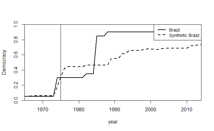
Ideally, the synthetic control group should be exactly like the treated unit through the entire pre-treatment period. This is important in that it makes us know whether SCM can actually reproduce the outcome of the treated unit if there had been no treatment. In other words, if there is any substantive effect of the treatment, we should see that large difference in the outcome between the treated unit and the control group only after the occurence of the treatment.
Now, we need to compute the estimate of the treatment effect for each period. We do this by subtracting the prediction for the control group from that of the treated unit. The gaps plot is simply the yearly difference between the treated unit (black line) and the synthetic control (straight horizontal line at zero).
gaps.plot(dataprep.res = dataprep.out.br.polity,
          synth.res = synth.out.br.polity,
          Ylab = c('Democracy'),
          Xlab = c('year')
)
abline(v = 1975)
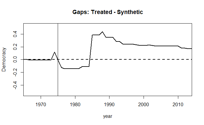
The figure above compares the evolution of democracy level between Brazil and the resulting synthetic control group. Substantively, this means that there was only a short-term effect of oil discovery on the level of democracy in Brazil. In addition to that, the path plot shows that despite a fall in the democracy level in relation to the synthetic control, Brazil overtook its counterpart.
Inference
Now that we have created the synthetic control group and estimated the treatment effect, the question remains how we can test for the statistical significance of the effect. As of now, there are no conventional statistical inference for synthetic control methods. So, we make use of test that are kind of intuitive, namely the placebo treatment effects of untreated units. There are two types of placebo tests: (1) Placebos in space (2) Placebos in time. The logic behind the placebo studies is that the impact of the event under analysis would not be credible if an estimated effect of similar or greater degree were observed in cases where the intervention did not occur.
In this analysis, I use in-space placebo tests to compare the estimated treatment effect for the treated Brazil with all the (fake) treatment effects of the control countries, obtained from experiments where each control country is presumably affected by the same event in the same year as the treated country. If the estimated effect in the treated Brazil is larger than the majority of the effects obtained by the (fake) experiments, one can conlcude that the baseline findings are not due to chance. If that were to be the case, we can attribute the effect to the peak of oil discovery. But note that the significance is contigent on the availabilty of a minimum of 19 units in the donor pool.
The next step is to take the outputs from dataprep and synth, and place them into the function generate.placebos(). It builds a synthetic control for each unit used in the donor pool.
tdf.polity <- generate.placebos(
  dataprep.out = dataprep.out.br.polity,
  synth.out = synth.out.br.polity)
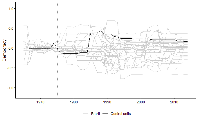
Then, we construct the gaps plot for the placebo units and Brazil. In the figure below, the black line represents the distance between the treated unit and its synthetic control. Each gray line shows the distance between a single unit in the donor pool and its own synthetic control.
plot.placebos.polity <- plot_placebos(tdf = tdf.polity,
                                      discard.extreme=T, ylab='Democracy')
plot.placebos.polity
The formalization of the placebo in space test can be done by creating a pre/post MSPE plot. MSPE (Mean Squared Prediction Error) measures the closeness of a synthetic control to the treated unit on the path of the outcome variable before the treatment. This is the quantity that the algorithm in Synth tries to reduce. We divide the post-treatment MSPE by the pre-treatment MSPE of each unit and their synthetic control. If the ratio for the treated unit is greater than that of all other (or 95%) placebos, we may conclude that we observe a treatment effect that exceeds what we should obtain by chance.
In the figure below, Brazil, which we identifed as showing a short-run negative effect of oil discovery on democracy, does not have a high ratio of the sample that corresponds to a p-value less than 0.05 (p-value = 35/51 > 0.05). This suggests that, in Brazil, oil discovery did not systematically influence democracy level.
plot.mspe.polity <- mspe.plot(tdf = tdf.polity)
plot.mspe.polity
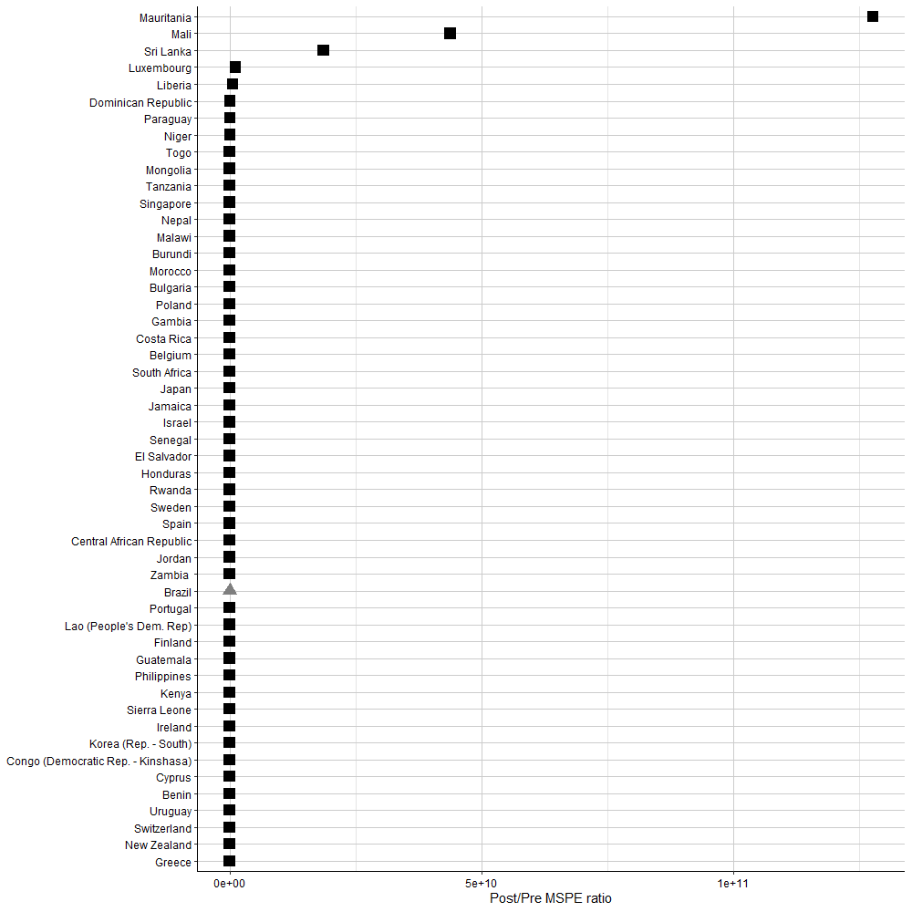
MSPE: Brazil and control countries.
Conclusion
In Masi and Ricciuti’s (2019) analysis of Brazil, the placebo tests and the implied p-values confirmed a significant short-run negative effect of oil discovery on democracy. But after the drop in the level of democracy compared to the synthetic control, Brazil overhauled its counterpart. Although we found a similar pattern in our result, our result lacks statistical significance.
It is important to also run sensitivity test in SCM. The first sensitivity test entails moving the intervention date. We could, for example, set the intervention date prior to or after the actual intervention date. Then we check if the treatment effect remains after this modification. A second sensitivity test is to verify whether our result is fairly robust to changes concerning how the control group is composed. The step is as follows: we re-run the synthetic control for the treated unit, but take away from the donor pools units that were initially used for its synthetic control one-at-a-time. If the effects disappear by dropping one of them, this could mean that the effect we get is merely a random variation due to one control.
Masi and Ricciuti (2019), for example, re-estimated Brazil synthetic control with this leave-one-out procedure. Then, they evaluated to what extent the findings were driven by a certain control country. The negative effect in Brazil is shorter due to the exclusion of the Democratic Republic of Congo, but, by excluding Portugal, a positive effect was observed! Although this procedure is likely to give up fit, it is a good way to minimize the chances that the results we get are caused by a single country in the donor pool that (un)democratized during the period of analysis.
Sources
- Abadie, Alberto (2021). “Using Synthetic Controls: Feasibility, Data Requirements, and Methodological Aspects.” Journal of Economic Literature 59(2), 391-425.
- Abadie, A., Diamond, A., & Hainmueller, J. (2015). Comparative Politics and the Synthetic Control Method. American Journal of Political Science, 59(2), 495–510.
- Abadie, Alberto, Diamond, A., & Hainmueller, J. (2011). Synth: An R Package for Synthetic Control Methods in Comparative Case Studies. Journal of Statistical Software, 42(13).
- Abadie, A., Diamond, A., & Hainmueller, J. (2010). Synthetic Control Methods for Comparative Case Studies: Estimating the Effect of California’s Tobacco Control Program. Journal of the American Statistical Association, 105(490), 493–505.
- Abadie, A., & Gardeazabal, J. (2003). The Economic Costs of Conflict: A Case Study of the Basque Country. American Economic Review, 93(1), 113–132.
- Castanho Silva, Bruno and Michael DeWitt (2020). “SCtools: Extensions for Synthetic Controls Analysis”. In: R package version 0.3.1.
- Masi, Tania, and Roberto Ricciuti (2019). “The Heterogeneous Effect of Oil Discoveries on Democracy.” Economics and Politics 31 (3): 374–402.
- PEP online course. Class 10: Synthetic control method
